Varying Fracface Pressure

More advanced use of bluebonnet.flow in a project where pressure variation at the frac-face or bottom-hole is approximately known.

%load_ext autoreload
%autoreload 2
import numpy as np
import pandas as pd
import matplotlib.pyplot as plt
from scipy import interpolate

from bluebonnet.flow import FlowProperties, SinglePhaseReservoir
from bluebonnet.fluids import build_pvt_gas
from bluebonnet.forecast.forecast_pressure import (
    fit_production_pressure,
    plot_production_comparison,
)
from bluebonnet import plotting

pressure_initial = 12_000.0
pressure_fracface = 5_000.0

n_times = 1_000
t_end = 20
time = np.linspace(0, np.sqrt(t_end), n_times) ** 2
pressure_v_time = np.full(n_times, pressure_fracface)
pressure_v_time[n_times // 4 : n_times // 2] /= 2.0
pressure_v_time[n_times // 2 :] /= 4.0

pvt_gas = pd.read_csv("../tests/data/pvt_gas.csv").rename(
    columns={
        "P": "pressure",
        "Z-Factor": "z-factor",
        "Cg": "compressibility",
        "Viscosity": "viscosity",
    }
)
flow_properties = FlowProperties(pvt_gas, pressure_initial)
pseudopressure_fracface = flow_properties.m_scaled_func(pressure_fracface)
pseudopressure_initial = flow_properties.m_scaled_func(pressure_initial)

print("mf =", flow_properties.m_scaled_func(pressure_fracface))

res = SinglePhaseReservoir(100, pressure_fracface, pressure_initial, flow_properties)

%time res.simulate(time, pressure_v_time)

recovery = res.recovery_factor()


def resource_left(pseudopressure, pvt):
    density = interpolate.interp1d(pvt.pvt_props["m-scaled"], pvt.pvt_props["Density"])
    print(max(pvt.pvt_props["m-scaled"]))
    p = np.minimum(pseudopressure, max(pvt.pvt_props["m-scaled"]))
    return (density(p)).sum(axis=1) / len(pseudopressure[0])


density_interp = interpolate.interp1d(
    flow_properties.pvt_props["m-scaled"], flow_properties.pvt_props["Density"]
)
remaining_gas = (resource_left(res.pseudopressure, flow_properties)) / (
    density_interp(pseudopressure_initial)
)
print(
    f"{pseudopressure_fracface=}",
    res.pseudopressure[-1][0],
    f"Deviation is {(recovery[-1] - 1 + remaining_gas[-1]) / recovery[-1] * 100:3.2g}%",
)
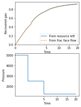
fig, (ax1, ax2) = plt.subplots(2, 1)
fig.set_size_inches(4, 6)
ax1.plot(time, 1 - remaining_gas, label="From resource left")
ax1.plot(time, recovery, "--", label="From frac face flow")
ax1.legend()
ax1.set(
    xlabel="Time",
    ylabel="Recovered gas",
    ylim=(0, None),
    xscale="squareroot",
    xlim=(0, None),
)

ax2.plot(time, pressure_v_time, label="Pressure")
ax2.set(xlabel="Time", xscale="squareroot", ylabel="Pressure");

mf = 0.09720937870967307
CPU times: user 3.08 s, sys: 11.7 ms, total: 3.09 s
Wall time: 3.09 s
0.3642368902150243
pseudopressure_fracface=array(0.09720938) 0.0008833922400551281 Deviation is  -1%

[Text(0.5, 0, 'Time'), None, Text(0, 0.5, 'Pressure')]

Build PVT data

There are two ways to create the necessary pressure-volume-temperature data.

1. Use the well data and an appropriate equation of state

2. Pull data from a pre-made csv file.

We will show both with the next code cell.

#
## Using the well data and bluebonnet.fluids
#
play = "HAYNESVILLE SHALE"
field_values = {
    "N2": 0.0,
    "H2S": 0.0,
    "CO2": 0.0002,
    "Gas Specific Gravity": 0.58,
    "Reservoir Temperature (deg F)": 285.21375,
}
gas_dryness = "wet gas"
pvt_gas = build_pvt_gas(field_values, gas_dryness)
# pvt_gas.to_csv("../tests/data/pvt_gas_" + Play + "_" + str(WellNumber) + ".csv")
print(pvt_gas.head())

#
## Using pre-gathered pvt data
#
pvt_gas = pd.read_csv("../tests/data/pvt_gas_" + play + "_20.csv", index_col=0)
pvt_gas

	temperature	pressure	Density	z-factor	compressibility	viscosity	pseudopressure
0	285.21375	10.0	0.021024	0.999592	0.100043	0.014638	0.000000e+00
1	285.21375	20.0	0.042065	0.999181	0.050043	0.014638	2.050874e+04
2	285.21375	30.0	0.063123	0.998775	0.033376	0.014639	5.470201e+04
3	285.21375	40.0	0.084198	0.998370	0.025043	0.014639	1.025897e+05
4	285.21375	50.0	0.105290	0.997967	0.020042	0.014640	1.641813e+05
...	...	...	...	...	...	...	...
1394	285.21375	13950.0	17.710554	1.655297	0.000029	0.029885	6.092847e+09
1395	285.21375	13960.0	17.715675	1.656005	0.000029	0.029895	6.098487e+09
1396	285.21375	13970.0	17.720791	1.656713	0.000029	0.029905	6.104126e+09
1397	285.21375	13980.0	17.725903	1.657421	0.000029	0.029915	6.109766e+09
1398	285.21375	13990.0	17.731011	1.658128	0.000029	0.029925	6.115405e+09

1399 rows × 7 columns

Fit wells

well_number = "20"
prod_file = f"../data/dataset_1_well_{well_number}.csv"
# This file contains pressure and production data. Rows 1 and 2 have information about units, so skip
prod = pd.read_csv(prod_file, skiprows=[1, 2]).rename(
    columns={
        "Time (Days)": "Days",
        "Gas Volume (MMscf)": "Gas",
        "Calculated Sandface Pressure  (psi(a))": "Pressure",
    }
)[["Days", "Gas", "Pressure"]]
# This file contains an estimate of initial pressure. That's all I need it for here.
well_file = f"../data/WellData_{well_number}.csv"
pressure_initial = float(
    pd.read_csv(well_file)
    .set_index("Field")
    .loc["Initial Pressure Estimate (psi)"]
    .iloc[0]
)

result = fit_production_pressure(
    prod,
    pvt_gas,
    pressure_initial,
    n_iter=40,
    pressure_imax=12000,
    filter_window_size=30,
    inplace_max=100000,
)
result

Fit Statistics

fitting method	Nelder-Mead
# function evals	101
# data points	416
# variables	3
chi-square	48434965.2
reduced chi-square	117275.945
Akaike info crit.	4858.65967
Bayesian info crit.	4870.75172

Variables

name	value	initial value	min	max	vary
tau	827.982319	830	30.0000000	830.000000	True
M	51957.6360	13864.498560000016	13850.5730	100000.000	True
p_initial	10389.2303	10000.0	9539.17738	12000.0000	True

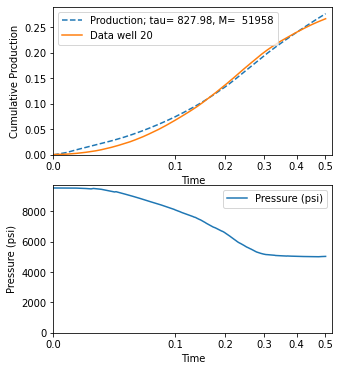
Plot the result

fig, (ax1, ax2) = plot_production_comparison(
    prod,
    pvt_gas,
    result.params,
    filter_window_size=30,
    well_name=f"Data well {well_number}",
)