Varying Fracface Pressure

More advanced use of bluebonnet.flow in a project where pressure variation at the frac-face or bottom-hole is approximately known.

You can download and run this notebook with jupyter by clicking on the “Edit on github” button in the upper right corner. Then, install bluebonnet with

pip install bluebonnet

or inside the notebook with

%pip install bluebonnet

and follow below

import numpy as np
import pandas as pd
import matplotlib.pyplot as plt
from scipy import interpolate

from bluebonnet.flow import FlowProperties, SinglePhaseReservoir
from bluebonnet.fluids import build_pvt_gas
from bluebonnet.forecast.forecast_pressure import (
    fit_production_pressure,
    plot_production_comparison,
)
from bluebonnet import plotting

pressure_initial = 12_000.0
pressure_fracface = 5_000.0

n_times = 1_000
t_end = 20
time = np.linspace(0, np.sqrt(t_end), n_times) ** 2
pressure_v_time = np.full(n_times, pressure_fracface)
pressure_v_time[n_times // 4 : n_times // 2] /= 2.0
pressure_v_time[n_times // 2 :] /= 4.0

pvt_gas = pd.read_csv(
    "https://raw.githubusercontent.com/frank1010111/bluebonnet/main/tests/data/pvt_gas.csv"
).rename(
    columns={
        "P": "pressure",
        "Z-Factor": "z-factor",
        "Cg": "compressibility",
        "Viscosity": "viscosity",
    }
)
flow_properties = FlowProperties(pvt_gas, pressure_initial)
pseudopressure_fracface = flow_properties.m_scaled_func(pressure_fracface)
pseudopressure_initial = flow_properties.m_scaled_func(pressure_initial)

print("mf =", flow_properties.m_scaled_func(pressure_fracface))

res = SinglePhaseReservoir(100, pressure_fracface, pressure_initial, flow_properties)

%time res.simulate(time, pressure_v_time)

recovery = res.recovery_factor()


def resource_left(pseudopressure, pvt):
    density = interpolate.interp1d(pvt.pvt_props["m-scaled"], pvt.pvt_props["Density"])
    print(max(pvt.pvt_props["m-scaled"]))
    p = np.minimum(pseudopressure, max(pvt.pvt_props["m-scaled"]))
    return (density(p)).sum(axis=1) / len(pseudopressure[0])


density_interp = interpolate.interp1d(
    flow_properties.pvt_props["m-scaled"], flow_properties.pvt_props["Density"]
)
remaining_gas = (resource_left(res.pseudopressure, flow_properties)) / (
    density_interp(pseudopressure_initial)
)
print(
    f"{pseudopressure_fracface=}",
    res.pseudopressure[-1][0],
    f"Deviation is {(recovery[-1] - 1 + remaining_gas[-1]) / recovery[-1] * 100:3.2g}%",
)
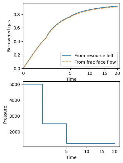
fig, (ax1, ax2) = plt.subplots(2, 1)
fig.set_size_inches(4, 6)
ax1.plot(time, 1 - remaining_gas, label="From resource left")
ax1.plot(time, recovery, "--", label="From frac face flow")
ax1.legend()
ax1.set(
    xlabel="Time",
    ylabel="Recovered gas",
    ylim=(0, None),
    xscale="squareroot",
    xlim=(0, None),
)

ax2.plot(time, pressure_v_time, label="Pressure")
ax2.set(xlabel="Time", xscale="squareroot", ylabel="Pressure");

mf = 0.09720937870967307
CPU times: user 2.03 s, sys: 5.49 ms, total: 2.03 s
Wall time: 2.04 s
0.3642368902150243
pseudopressure_fracface=array(0.09720938) 0.0008833922400551281 Deviation is  -1%

Build PVT data

There are two ways to create the necessary pressure-volume-temperature data.

1. Use the well data and an appropriate equation of state

2. Pull data from a pre-made csv file.

We will show both with the next code cell.

# #########################
# Haynesville shale gas play
# Using the well data and bluebonnet.fluids
# #########################
field_values = {
    "N2": 0.0,
    "H2S": 0.0,
    "CO2": 0.0002,
    "Gas Specific Gravity": 0.58,
    "Reservoir Temperature (deg F)": 285.21375,
}
gas_dryness = "wet gas"
pvt_gas = build_pvt_gas(field_values, gas_dryness)


# #########################
# Or, you could using pre-gathered pvt data
# #########################
# pvt_gas = pd.read_csv("https://raw.githubusercontent.com/frank1010111/bluebonnet/main/tests/data/pvt_gas_HAYNESVILLE%20SHALE_20.csv", index_col=0)

print(pvt_gas.head())

   temperature  pressure   Density  z-factor  compressibility  viscosity  \
0    285.21375      10.0  0.021024  0.999592         0.100043   0.014638   
1    285.21375      20.0  0.042065  0.999181         0.050043   0.014638   
2    285.21375      30.0  0.063123  0.998775         0.033376   0.014639   
3    285.21375      40.0  0.084198  0.998370         0.025043   0.014639   
4    285.21375      50.0  0.105290  0.997967         0.020042   0.014640   

   pseudopressure  
0        0.000000  
1    20508.736605  
2    54702.013998  
3   102589.697359  
4   164181.289746  

Fit wells

well_number = "20"
prod_file = f"https://raw.githubusercontent.com/frank1010111/bluebonnet/main/data/dataset_1_well_{well_number}.csv"
# This file contains pressure and production data. Rows 1 and 2 have information about units, so skip
prod = pd.read_csv(prod_file, skiprows=[1, 2]).rename(
    columns={
        "Time (Days)": "Days",
        "Gas Volume (MMscf)": "Gas",
        "Calculated Sandface Pressure  (psi(a))": "Pressure",
    }
)[["Days", "Gas", "Pressure"]]
# This file contains an estimate of initial pressure. That's all I need it for here.
well_file = f"https://media.githubusercontent.com/media/frank1010111/bluebonnet/main/data/WellData_{well_number}.csv"
pressure_initial = float(
    pd.read_csv(well_file)
    .set_index("Field")
    .loc["Initial Pressure Estimate (psi)"]
    .iloc[0]
)

result = fit_production_pressure(
    prod,
    pvt_gas,
    pressure_initial,
    n_iter=40,
    pressure_imax=12000,
    filter_window_size=30,
    inplace_max=100000,
)
result

Fit Statistics

fitting method	Nelder-Mead
# function evals	41
# data points	416
# variables	3
chi-square	52336113.5
reduced chi-square	126721.824
Akaike info crit.	4890.88497
Bayesian info crit.	4902.97702

Variables

name	value	initial value	min	max	vary
tau	829.929628	830	30.0000000	830.000000	True
M	52545.0889	13864.498560000016	13850.5730	100000.000	True
p_initial	10403.8830	10000.0	9539.17738	12000.0000	True

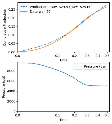
Plot the result

fig, (ax1, ax2) = plot_production_comparison(
    prod,
    pvt_gas,
    result.params,
    filter_window_size=30,
    well_name=f"Data well {well_number}",
)