Fitting and forecasting
To use bluebonnet.forecast in a project:
[1]:
import matplotlib.pyplot as plt
import numpy as np
import pandas as pd
from scipy.integrate import cumulative_trapezoid
from scipy.interpolate import interp1d

from bluebonnet.flow import (
    FlowProperties,
    IdealReservoir,
    RelPermParams,
    SinglePhaseReservoir,
)
from bluebonnet.forecast import ForecasterOnePhase
Forecasting with an ideal gas
[2]:
# Get ideal gas recovery
t_end = 6
nx = 50
pressure_initial = 9000
pressure_bh = 1000
time = np.linspace(0, np.sqrt(t_end), 10_000) ** 2
res_ideal = IdealReservoir(nx, pressure_bh, pressure_initial, None)
res_ideal.simulate(time)
rf_ideal = res_ideal.recovery_factor()
rf_func = interp1d(time, rf_ideal, bounds_error=False, fill_value=(0, rf_ideal[-1]))
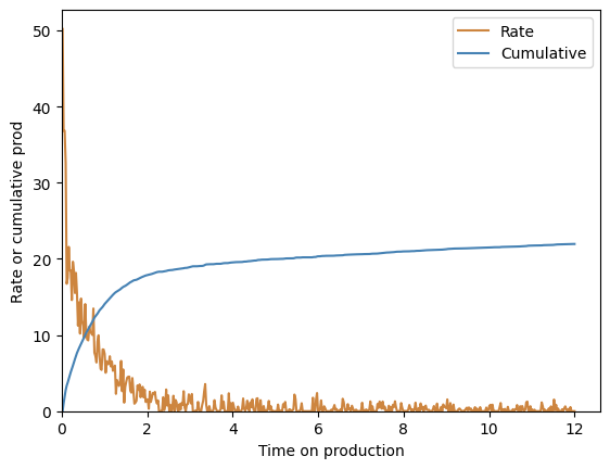
[3]:
# Create test production to fit to
m_factor = 1e3
fake_tau = 2
time_on_production = np.linspace(1e-2, t_end, 500) * fake_tau

# Add some randomness to make this interesting
randomness = np.random.default_rng(42).normal(0, 2e-3, size=len(time_on_production)) / np.sqrt(
    time_on_production + 0.1
)
fake_rf = rf_func(time_on_production / fake_tau)
fake_rate = m_factor * np.maximum(np.gradient(fake_rf) + randomness, 0)
cum_production = cumulative_trapezoid(fake_rate, time_on_production, initial=0)

fig, ax = plt.subplots()
ax.plot(time_on_production, fake_rate, color="peru", label="Rate")
ax.plot(time_on_production, cum_production, color="steelblue", label="Cumulative")
ax.set(
    xlabel="Time on production",
    ylabel="Rate or cumulative prod",
    xlim=(0, None),
    ylim=(0, None),
)
ax.legend()
[3]:
<matplotlib.legend.Legend at 0x787b415b2c30>
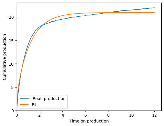
After that setup, the actual fitting is fairly simple:
[4]:
# Fit the test production
scaling_curve = ForecasterOnePhase(rf_func)

scaling_curve.fit(time_on_production, cum_production)
M_fit = scaling_curve.M_
tau_fit = scaling_curve.tau_
print(f"{tau_fit=:.2f}, and should be {fake_tau}")
tau_fit=2.84, and should be 2
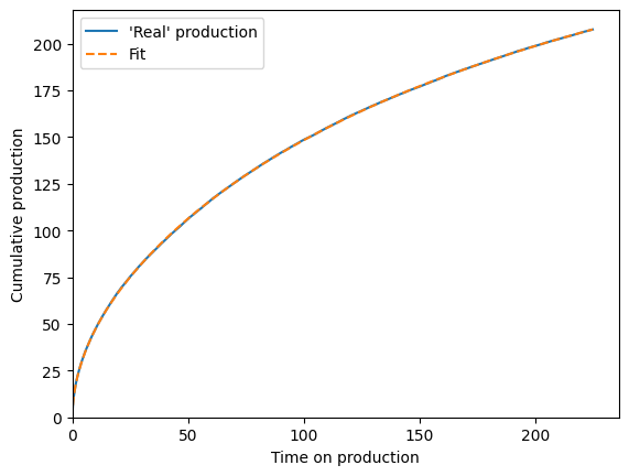
[5]:
# Forecast cumulative production and compare fit
cum_bestfit = scaling_curve.forecast_cum(time_on_production)

fig, ax = plt.subplots()
ax.plot(time_on_production, cum_production, label="'Real' production")
ax.plot(time_on_production, cum_bestfit, label="Fit")
ax.legend()
ax.set(
    xlim=(0, None),
    ylim=(0, None),
    xlabel="Time on production",
    ylabel="Cumulative production",
);
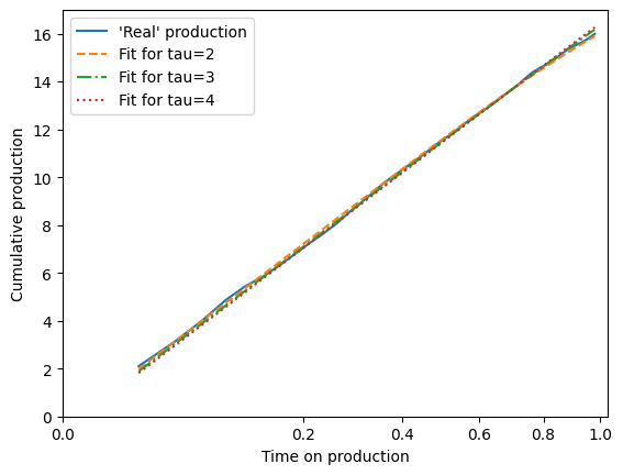
The forecaster also allows you to fit production with a known value for \(\tau\). This is important when the well has not yet ended transient flow, usually around \(t < 0.5\tau\). Until that point, setting \(\tau\) to any value above a certain point will achieve the same fit but different in-place and ultimate recovery estimates.
A few example fits:
[6]:
from itertools import cycle

cum_production = cum_production[time_on_production < 1] + 2.1
time_on_production = time_on_production[time_on_production < 1]

fig, ax = plt.subplots()

lines = ["--", "-.", ":"]
linecycler = cycle(lines)
ax.plot(time_on_production, cum_production, label="'Real' production")
for tau in [2, 3, 4]:
    scaling_curve.fit(time_on_production, cum_production, tau=tau)
    M_fit = scaling_curve.M_
    print(f"{tau=:.2f}, and {M_fit=:.2f}")

    # Forecast cumulative production and compare fit
    cum_bestfit = scaling_curve.forecast_cum(time_on_production)
    ax.plot(time_on_production, cum_bestfit, next(linecycler), label=f"Fit for {tau=}")
ax.legend()
ax.set(
    xlim=(0, None),
    ylim=(0, None),
    xlabel="Time on production",
    ylabel="Cumulative production",
    xscale="squareroot",
);
tau=2.00, and M_fit=24.05
tau=3.00, and M_fit=29.37
tau=4.00, and M_fit=34.06
Forecasting with a real gas
[7]:
pvt_gas = pd.read_csv(
    "https://raw.githubusercontent.com/frank1010111/bluebonnet/main/tests/data/pvt_gas.csv"
).rename(
    columns={
        "P": "pressure",
        "Z-Factor": "z-factor",
        "Cg": "compressibility",
        "Viscosity": "viscosity",
        "Density": "density",
    }
)
t_end = 6
nx = 60
pressure_initial = 12_000
pressure_bh = 1000
real_gas_flow_props = FlowProperties(pvt_gas, p_i=pressure_initial)
time = np.linspace(0, np.sqrt(t_end), 10_000) ** 2
res_real = SinglePhaseReservoir(nx, pressure_bh, pressure_initial, real_gas_flow_props)
res_real.simulate(time)
rf_real = res_real.recovery_factor()
[8]:
fake_ogip = 300
fake_tau = 150
time_on_production = time[: len(time) // 2] * fake_tau
randomness = np.maximum(
    0, np.random.default_rng(42).normal(0, 0.02, size=len(time_on_production))
).cumsum()
fake_cum = rf_real[: len(time) // 2] * fake_ogip + randomness
[9]:
rf_func = interp1d(time, rf_real, bounds_error=False, fill_value=(0, rf_real[-1]))
scaling_curve = ForecasterOnePhase(rf_func)
scaling_curve.fit(time_on_production, fake_cum)
print(
    f"The fitted OOIP is {scaling_curve.M_:.2f}, and it should be over {fake_ogip} "
    "(because all the randomness is positive)\n"
    f"The fitted tau is {scaling_curve.tau_:.2f}, and it should be near {fake_tau}"
)

cum_bestfit = scaling_curve.forecast_cum(time_on_production)

fig, ax = plt.subplots()
ax.plot(time_on_production, fake_cum, label="'Real' production")
ax.plot(time_on_production, cum_bestfit, "--", label="Fit")
ax.legend()
ax.set(
    xlim=(0, None),
    ylim=(0, None),
    xlabel="Time on production",
    ylabel="Cumulative production",
);
The fitted OOIP is 389.75, and it should be over 300 (because all the randomness is positive)
The fitted tau is 175.52, and it should be near 150
Forecasting oil
Oil wells tend to be producing three phases at a time. Let’s say that the water phase is constant, and we can just worry about matching hydrocarbon production. These wells are almost all producing at below the bubble point, so a two-phase model is most appropriate.
[10]:
from bluebonnet.flow import (
    FlowPropertiesTwoPhase,
    relative_permeabilities,
)

# set conditions
Sw = 0.1
p_frac = 1000
p_res = 6_000
phi = 0.1

df_pvt_mp = pd.read_csv("../tests/data/pvt_multiphase_oil.csv")
relperm_params = RelPermParams(
    n_o=1, n_g=1, n_w=1, S_or=0, S_gc=0, S_wc=0.1, k_ro_max=1, k_rw_max=1, k_rg_max=1
)
saturations_test = pd.DataFrame(
    {"So": np.linspace(0, 0.9), "Sw": np.full(50, 0.1), "Sg": np.linspace(0.9, 0)}
)
kr_matrix = pd.DataFrame(
    relative_permeabilities(saturations_test.to_records(index=False), relperm_params)
)
df_kr = pd.concat([saturations_test, kr_matrix], axis=1)
reference_densities = {"rho_o0": 141.5 / (45 + 131.5), "rho_g0": 1.03e-3, "rho_w0": 1}
flow_props = FlowPropertiesTwoPhase.from_table(
    df_pvt_mp, df_kr, reference_densities, phi, Sw, p_res
)

# get recovery factor curve
res = SinglePhaseReservoir(50, p_frac, p_res, flow_props)
res.simulate(time)
rf_twophase = res.recovery_factor()
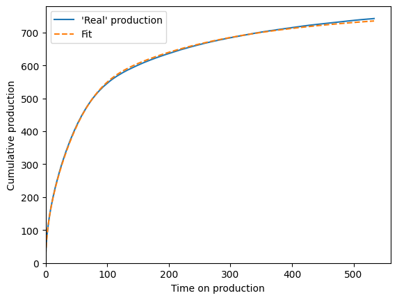
At this point, you have a recovery factor curve and can proceed just like real gas or ideal gas
[11]:
fake_ooip = 700
fake_tau = 200
time_on_production = time[: round(len(time) / 1.5)] * fake_tau
randomness = np.maximum(
    0, np.random.default_rng(42).normal(0, 0.02, size=len(time_on_production))
).cumsum()
fake_cum = rf_twophase[: round(len(time) / 1.5)] * fake_ooip + randomness
[12]:
rf_func = interp1d(time, rf_twophase, bounds_error=False, fill_value=(0, rf_twophase[-1]))
scaling_curve = ForecasterOnePhase(rf_func)
scaling_curve.fit(time_on_production, fake_cum)
print(
    f"The fitted OOIP is {scaling_curve.M_:.2f}, and it should be over {fake_ooip} "
    "(because all the randomness is positive)\n"
    f"The fitted tau is {scaling_curve.tau_:.2f}, and it should be near {fake_tau}"
)

cum_bestfit = scaling_curve.forecast_cum(time_on_production)

fig, ax = plt.subplots()
ax.plot(time_on_production, fake_cum, label="'Real' production")
ax.plot(time_on_production, cum_bestfit, "--", label="Fit")
ax.legend()
ax.set(
    xlim=(0, None),
    ylim=(0, None),
    xlabel="Time on production",
    ylabel="Cumulative production",
);
The fitted OOIP is 751.99, and it should be over 700 (because all the randomness is positive)
The fitted tau is 217.50, and it should be near 200