Getting Started with bluebonnet

Quick start

In your command line, run this:

pip install bluebonnet

Pip will automatically download the project dependencies and make bluebonnet available in your python environment.

Now, in your script or notebook, let’s import what we need:

import matplotlib.pyplot as plt
import numpy as np
from scipy.interpolate import interp1d

from bluebonnet.flow import IdealReservoir
from bluebonnet.forecast import Bounds, ForecasterOnePhase
from bluebonnet.plotting import (
    plot_pseudopressure,
    plot_recovery_factor,
    plot_recovery_rate,
)

Reservoir

First we need fluid properties. For absolute starters, let’s say we have an ideal gas. Our initial reservoir pressure is 9,000 psi, and we our frac-face pressure is 1,000 psi. Then, we build our reservoir:

initial_pressure = 9000
frac_face_pressure = 1000
num_points = 50
reservoir = IdealReservoir(num_points, frac_face_pressure, initial_pressure)

Then, simulate the reservoir drawdown:

num_time = 10_000
time_end = 6
time = np.linspace(0, np.sqrt(time_end), num_time) ** 2
reservoir.simulate(time)
fig, ax = plt.subplots()
plot_pseudopressure(reservoir, every=50, ax=ax);

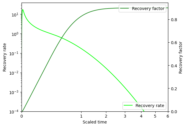
And calculate the recovery rate and recovery factor over time:

rf = reservoir.recovery_factor()
fig, ax = plt.subplots()
plot_recovery_rate(reservoir, ax, plot_kwargs={"color": "lime"})
ax.legend(loc="lower right")
ax2 = ax.twinx()
plot_recovery_factor(reservoir, ax2, plot_kwargs={"color": "forestgreen"})
ax2.legend(loc="upper right");

Fit and forecast a well

Now, to fit and forecast production from our well. Let’s use a synthetic well here:

fake_ooip = 100
fake_tau = 1.5
time_on_production = time[: len(time) // 2] * fake_tau
randomness = np.maximum(
    0, np.random.default_rng(42).normal(0, 0.02, size=len(time_on_production))
).cumsum()
fake_cum = rf[: len(time) // 2] * fake_ooip + randomness

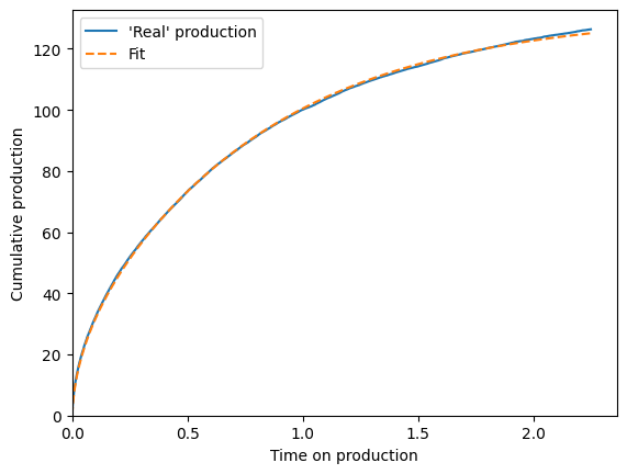
And then use ForecasterOnePhase to match its production:

rf_func = interp1d(time, rf, bounds_error=False, fill_value=(0, rf[-1]))
bounds = Bounds(M=(0, 500), tau=(0.1, 25))
scaling_curve = ForecasterOnePhase(rf_func, bounds)
scaling_curve.fit(time_on_production, fake_cum)
print(
    f"The fitted OOIP is {scaling_curve.M_:.2f}, and it should be over {fake_ooip} "
    "(because all the randomness is positive)\n"
    f"The fitted tau is {scaling_curve.tau_:.2f}, and it should be near {fake_tau}"
)


cum_bestfit = scaling_curve.forecast_cum(time_on_production)

fig, ax = plt.subplots()
ax.plot(time_on_production, fake_cum, label="'Real' production")
ax.plot(time_on_production, cum_bestfit, "--", label="Fit")
ax.legend()
ax.set(
    xlim=(0, None),
    ylim=(0, None),
    xlabel="Time on production",
    ylabel="Cumulative production",
);

The fitted OOIP is 146.25, and it should be over 100 (because all the randomness is positive)
The fitted tau is 1.85, and it should be near 1.5

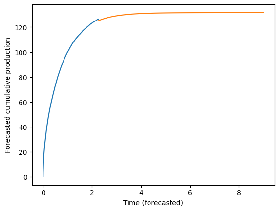
Then, forecast the future:

time_forecast = np.linspace(max(time_on_production), 9, 12 * 9)
forecast_cum = scaling_curve.forecast_cum(time_forecast)
fig, ax = plt.subplots()
ax.plot(time_on_production, fake_cum, label="'Real' production")
ax.plot(time_forecast, forecast_cum, scalex="squareroot")
ax.set(
    xlabel="Time (forecasted)",
    ylabel="Forecasted cumulative production",
);